My country, Colombia. Watch it!

The Republic of Colombia includes the northwestern part of South America. It is situated within the tropical zone, and is bounded on the north by the Caribbean Sea on the east by Venezuela and Brazil, Ecuador and Peru south and west by the Pacific Ocean and the Republic of Panama.

ITERATIVE METHODS FOR SOLVING SYSTEMS OF LINEAR EQUATIONS

Iterative method

In computational mathematics, an iterative method attempts to solve a problem (for example, finding the root of an equation or system of equations) by finding successive approximations to the solution starting from an initial guess. This approach is in contrast to direct methods, which attempt to solve the problem by a finite sequence of operations, and, in the absence of rounding errors, would deliver an exact solution (like solving a linear system of equations Ax = b by Gaussian elimination). Iterative methods are usually the only choice for nonlinear equations. However, iterative methods are often useful even for linear problems involving a large number of variables (sometimes of the order of millions), where direct methods would be prohibitively expensive (and in some cases impossible) even with the best available computing power.

*GAUSS-SEIDEL

Gauss sediel

View more presentations from jorgeduardooo.

*METHOD OF JACOBI

METHOD OF JACOBI

View more presentations from jorgeduardooo.

REFERENCES:

(1)NUMERICAL METHODS FOR ENGINEERS WITH PERSONAL COMPUTER APPLICATIONS. STEVEN C. Chapra / Raymond P. CANALE

(2) internet-google.

(3)Enciclopedia libre wikipedia

LU decomposition

LU decomposition

This type of factorization is useful for solving systems of equations.
Resume Gaussian elimination process applied to the matrix.

In linear algebra, the LU decomposition is a matrix decomposition which writes a matrix as the product of a lower triangular matrix and an upper triangular matrix. The product sometimes includes a permutation matrix as well. This decomposition is used in numerical analysis to solve systems of linear equations or calculate the determinant.

Lu decomposition

View more documents from jorgeduardooo.

REFERENCES:

(1)NUMERICAL METHODS FOR ENGINEERS WITH PERSONAL COMPUTER APPLICATIONS. STEVEN C. Chapra / Raymond P. CANALE

(2) internet-google.

(3)Enciclopedia libre wikipedia

METHODS FOR THE SOLUTION OF SYSTEMS OF EQUATIONS.

The matrix algebra is used to solve systems of linear equations. In fact it is used in various mathematical procedures as the solution of a set of nonlinear equations, interpolation, integration and differentiation which are reduced to a set of linear equations.

SIMPLE GAUSS

The method of Gauss to be the German mathematician Johann Carl Friedrich Gauss, is a generalization of the reduction method, which we use to eliminate an unknown quantity in the systems of two equations with two unknowns. It consists of the successive application of the method of reduction, using the criteria of equivalence of systems, to transform the augmented matrix with independent terms in a triangular matrix, so that each row (equation) have a mystery unless the immediately preceding . This provides a system, which we call step, such that the last equation has a single unknown, the last but two unknowns, the penultimate three unknowns, ..., and the first all unknowns.

The operations we can do this matrix to transform the initial system into an equivalent are:

• Multiply or divide a row by a nonzero real number.
• Add or subtract a row another row.
• Add a row another row multiplied by a nonzero number.
• Change the order of the rows.
• Change the order of the columns that correspond to the unknowns of the system taking into account the changes made at the time of writing the new equivalent.
• Delete rows that are proportional or linear combination of others.
• Delete rows zero (0 0 0 ... 0).

See the example in the following document..

Example method of gauss

View more documents from jorgeduardooo.

GAUSS-JORDAN

This method is a variant of Gauss elimination method. The main difference with this is that when a mystery is removed from an equation in the Gauss-Jordan, this is eliminated in all equations of the system rather than being limited to the subsequent equations.

The method generates an identity matrix and therefore do not need the back substitution process. It should be noted that the method can present the same difficulties that the method of simple Gaussian elimination.

Gauss jordan

View more presentations from jorgeduardooo.

SPECIAL METHODS

Arrays are widely used in computing, ease and lightness to manipulate information. In this context, the best way to represent graph, and are widely used in the numerical calculation.

Attached is a presentation with an explanation and rationale of two methods empeciales:

• Thomas Method
• Cholesky Method

These two methods are easy to program in any programming language, Microsoft Excel is recommended.

Cholesky method and Thomas

View more presentations from jorgeduardooo.

REFERENCES:

(1)NUMERICAL METHODS FOR ENGINEERS WITH PERSONAL COMPUTER APPLICATIONS. STEVEN C. Chapra / Raymond P. CANALE

(2) internet-google.

(3)Enciclopedia libre wikipedia

Basic concepts. Systems of equations

Before continuing our study of systems of equations is necessary to consider some concepts on determinants and matrices. Mathematical operations, etc.

Basic concepts. Systems of equations

View more presentations from jorgeduardooo.

REFERENCES:

(1)NUMERICAL METHODS FOR ENGINEERS WITH PERSONAL COMPUTER APPLICATIONS. STEVEN C. Chapra / Raymond P. CANALE

(2) internet-google.

(3)Enciclopedia libre wikipedia

SYSTEMS OF LINEAR EQUATIONS

Systems of linear equations

In mathematics and linear algebra, a system of linear equations, also known as linear system of equations or simply linear system is a set of linear equations over a field or a commutative ring. An example of linear system of equations is as follows:

The problem is to find the unknown values of the variables x1, x2 and x3 that satisfy the three equations.

SYSTEM TYPES

Systems of equations can be classified according to the number of solutions that may occur. According to that case may have the following cases:

• Incompatible system if it has no solution.
• System compatible if you have any solution in this case can also distinguish between:

-Determined when compatible system has a finite number of solutions.
-Compatible system supports indefinite when an infinite set of solutions.

Staying well classification:



REFERENCES:

(1)NUMERICAL METHODS FOR ENGINEERS WITH PERSONAL COMPUTER APPLICATIONS. STEVEN C. Chapra / Raymond P. CANALE

(2) internet-google.

(3)Enciclopedia libre wikipedia

CALCULATION OF MULTIPLE ROOTS AND COMPLEX ROOTS

CALCULATION OF MULTIPLE ROOTS AND COMPLEX ROOTS

When there are complex roots closed methods can not be used as the criterion for defining the range is the sign change does not apply to complex values.

For this reason, special methods have been developed to find real and complex roots of polynomials.

• MULLER'S METHOD
• THE BAIRSTOW METHOD

*MULLER METHOD:

The secant method obtains an approximation of the root leading a straight line to the axis X with two values of the function. Muller's method is similar, but building a parabola with three points.

The method consists of obtaining the coefficients of the parabola through the three points. These coefficients are used in the quadratic formula to get the value where the parabola intersects the X axis, ie the estimated result.

Once you know the approximate coefficients found through the root of the quadratic equation where:



Having to solve the quadratic to find the new result leaves open the possibility that complex roots can be calculated, where i = root of -1.

As a general rule is to choose the root whose discriminant D1 or D2
is the largest since this ensures that the new root is closest to the initial values proposed










*Bairstow Method

NUMERICAL METHODS

View more presentations from jorgeduardooo.

REFERENCES:

(1)NUMERICAL METHODS FOR ENGINEERS WITH PERSONAL COMPUTER APPLICATIONS. STEVEN C. Chapra / Raymond P. CANALE

(2)http://www.concepcionabraira.info/wp/?p=305

(3) internet-google.

(4)Enciclopedia libre wikipedia

PPTX ESTATE PRESENTATION EQUATIONS

The following document is in Spanish because of its extension

Busqueda de una raiz-Metodos numericos

View more presentations from jorgeduardooo.

METHODS USED FOR THE CALCULATION OF ROOTS OF EQUATIONS

METHODS USED FOR THE CALCULATION OF ROOTS OF EQUATIONS

 Graphical Methods
 Closed methods
 Open methods

Graphical Method:

Is to plot the function and see where it crosses the x-axis This item, which represents the value of X for which f (x) = 0 provides an initial approximation of the root.

• If in an interval [a.b] closed marks
f (a) * f (b)> 0 then we have: there are no roots or is an even number of them.

• If in an interval [a.b] closed marks
f (a) * f (b) <0>

Closed methods: bisection, false position.


*Bisection method:

The purpose of the method is to divide an interval always half in successive iterations to investigate the change of sign.

Suppose we want to solve the equation f (x) = 0 (where f is continuous. Given two points a and b such that f (a) f (b) have opposite signs, we know from Bolzano's theorem that f must have at least a root in the interval [a, b]. The bisection method divides the interval into two, using a third point c = (a + b) / 2.

At this time, there are two possibilities: f (a) f (c ), or f (c) and f (b) have opposite signs. The bisection algorithm is applied to the subinterval where the sign change occurs.
The bisection method is less efficient than Newton's method, but is much safer to ensure convergence.


Convergence is guaranteed if f (a) f (b) have opposite signs.

1. Is to find an interval (a, b) to ensure that the function root.
2. Find the midpoint of the interval, taking the point of bisection (c) as a proxy for the desired root.
3. It then identifies which of the two intervals is the root. Choose between (a, c) and (c, b), a range in which the function changes sign.
4. We review the stopping criterion. The process is repeated n times, until the bisection point (c) practically coincides with the exact value of the root.

*FALSE POSITION METHOD

It is practically the same method but has a bisection difference.
Instead of using a point intersection method is used on a line with the axis x. Then using similar triangles we have:




The algorithm is getting on at every step a smaller interval that includes a root of the function f

OPEN METHOD: FIXED POINT, NEWTON RAPHSON, SECANT.

*FIXED POINT METHOD

This method is based on obtained from the equation f (x) = 0 an equivalent equation of the form g (x) = x whose solution becomes a fixed point of ge iterating from an initial value until it reaches.

This method is applied to solve equations of the form

x = g (x)

If the equation is f (x) = 0 then can be solved for x or else add x on both sides of the equation to put it in an appropriate manner.

For example: x2-2x+3=0 is fixed for X=x2+3/2

*NEWTON RAPHSON METHOD

The Newton-Raphson method is an open, in the sense that their global convergence is not guaranteed. The only way to achieve convergence is to select an initial value close enough to the desired root. Thus, we must start the iteration with a value reasonably close to zero (called the starting point or assumption).

The relative proximity of the starting point to the root of much depends on the nature of the function itself, if it shows multiple points of inflection or large earrings in the vicinity of the root, then the probability that the algorithm diverges increase, which requires selecting an assumed value close to the root.
Once this is done, the method linearizes the function by the tangent line at that assumption. The abscissa at the origin of this line will be, according to the method, a better approximation of the root as the previous value.

Will successive iterations until the method has converged sufficiently.

STEPS

 1. Taking F (x) = 0 calculate the derivative of the function symbolically.
 2. Choose an initial value, xi.
 3. Find Xi +1 through Newton-Raphson formula.
 4. Calculate% Ea.
 5. Ea ≤% If% Then we report the results of the root, otherwise make the calculated +1 xi xi is the new and return to step 3.




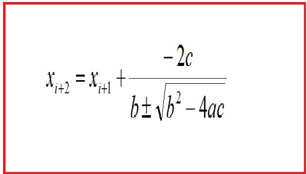
SECANT METHOD

In numerical analysis of the secant method is a method for finding the zeros of a function in an iterative fashion.

It is a variation of Newton-Raphson method where instead of calculating the derivative of the function at the point of study, bearing in mind the definition of derivative, the slope is close to the line that connects the function evaluated at the point of study and the point from the previous iteration. This method is especially relevant when the computational cost of deriving the function of study and evaluate is too high, so Newton's method is not attractive.



REFERENCES:

(1)NUMERICAL METHODS FOR ENGINEERS WITH PERSONAL COMPUTER APPLICATIONS. STEVEN C. Chapra / Raymond P. CANALE

(2)http://www.concepcionabraira.info/wp/?p=305

(3) internet-google.

(4)Enciclopedia libre wikipedia